LatentWorld
Published in Publications, 2026
LatentWorld: Exploration of Latent Space Phase Transitions as a way of generating novel Images
Ricardo Mehl
MA Design for Digital Futures, Nuremberg Institute of Technology Georg Simon Ohm
mehlri77989@th-nuernberg.de
Introduction/Related Work: The Landscape of Latent Spaces
The latent space in generative models like Stable Diffusion is a compressed, abstract representation of high-dimensional image data encoded in tandem with semantic concepts from training into a lower-dimensional space. This space can be described as a navigable map: similar images or ideas cluster nearby, enabling the decoder to reconstruct visuals from targeted points, which users typically steer toward using text prompts.
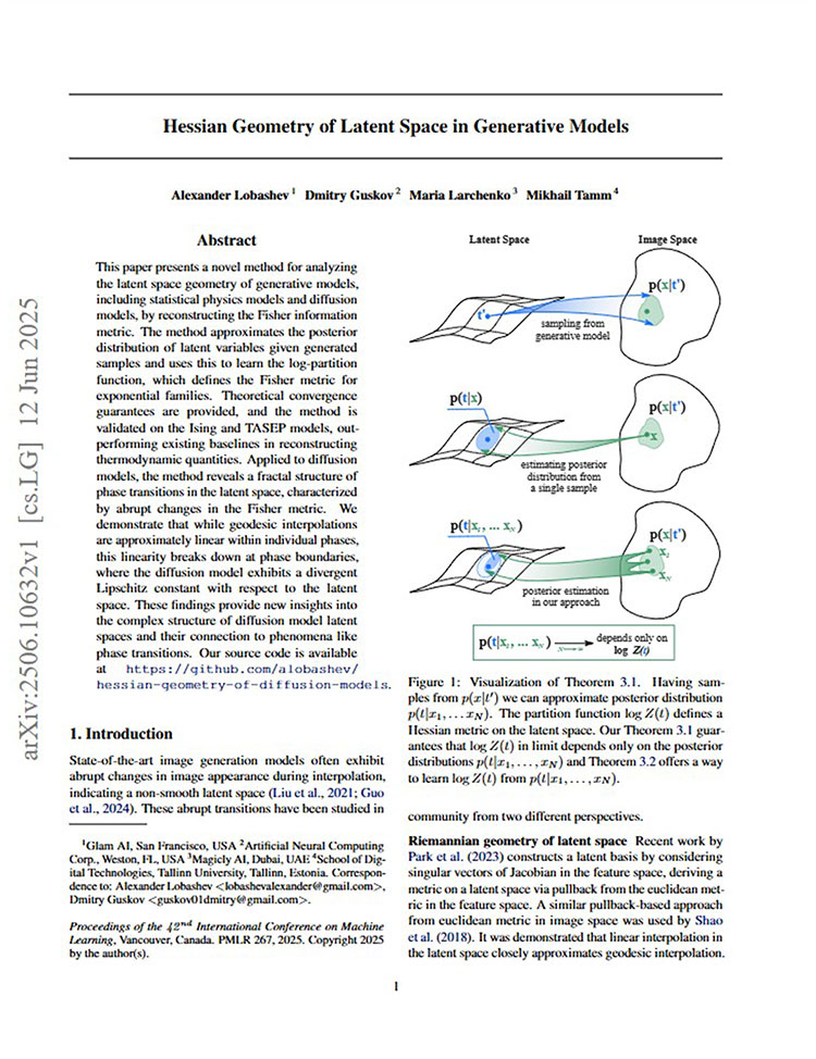
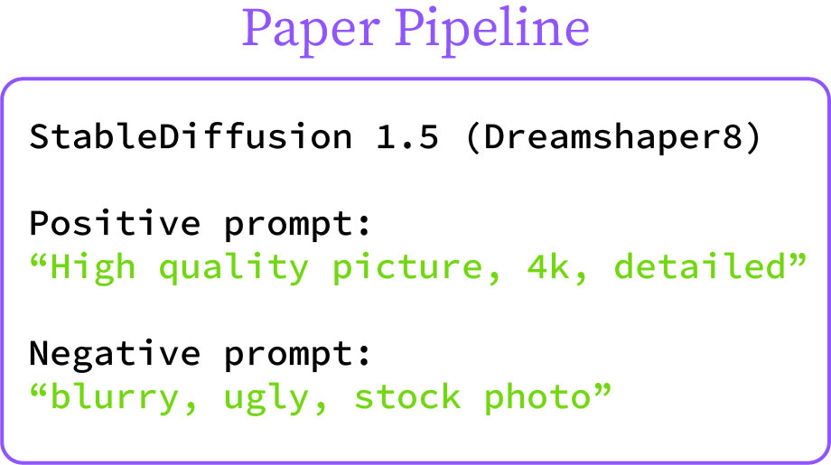
This project builds on the approach in Lobashev, A., Guskov, D., Larchenko, M., & Tamm, M. (2025). Hessian Geometry of Latent Space in Generative Models, which conceptualizes latent space exploration as navigating a country. Their exploration was deliberately neutral, employing minimal guidance to unveil the latent space’s inherent geometry without targeted semantic steering. Using Stable Diffusion 1.5 with generic prompts such as “High quality picture, 4k, detailed” and negative prompts such as “blurry, ugly, stock photo,” the authors let the model’s training biases surface organically. By scattering a two-dimensional grid of latents, they analyzed the space’s geometry, uncovering phase transitions between semantic concepts such as “cat” and “mountain.” These transitions manifest as rifts where the diffusion model becomes unstable, generating fractal patterns of either concept that extend to the model’s bit-level resolution. Notably, interpolations within certain rifts introduce emergent third concepts, such as “car,” highlighting the latent space’s intricate, non-linear structure.
Implications: Semantic Archipelagos
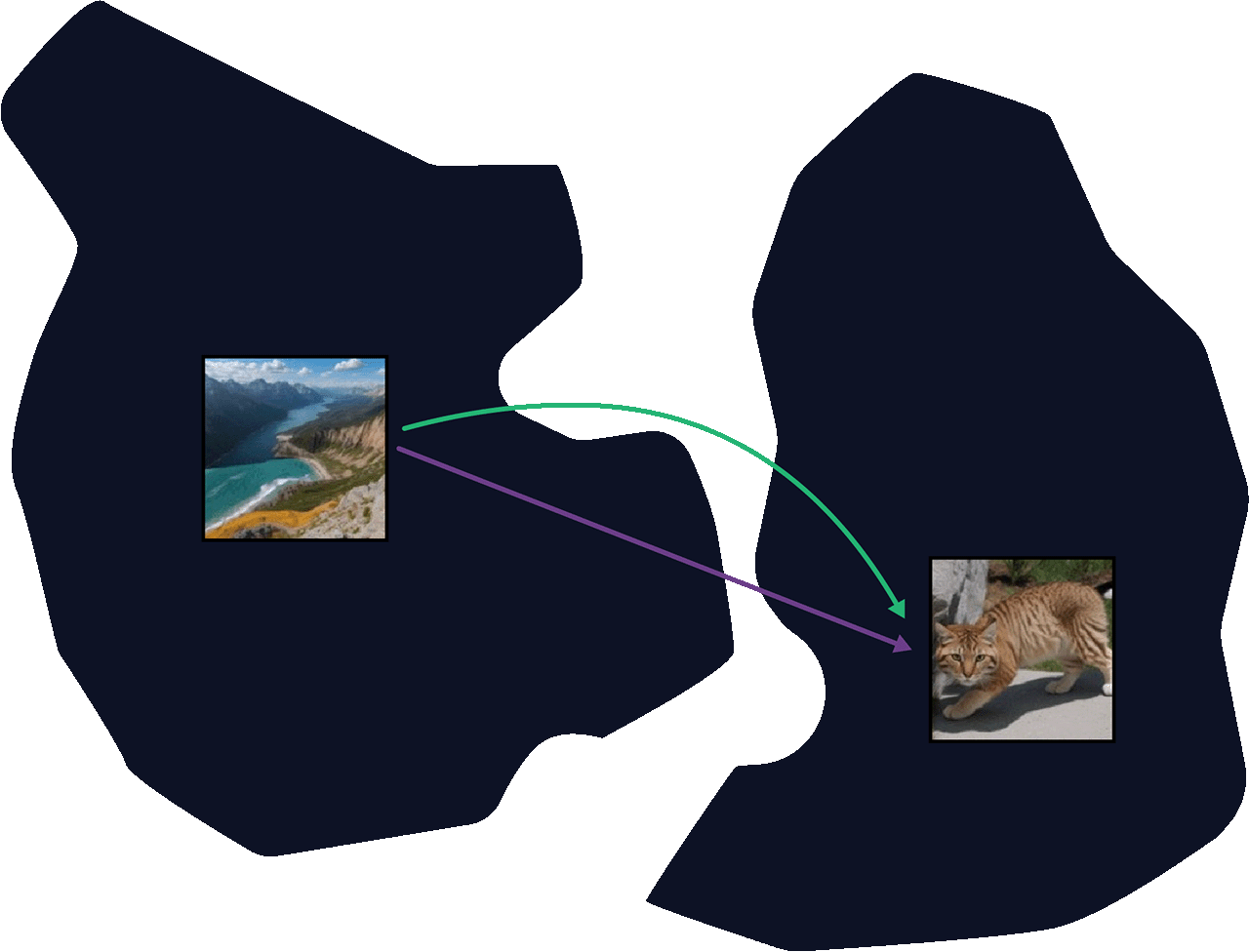
The implications suggest that no clear semantic bridge exists between concepts like “cat” and “mountain.” My hypothesis is that because human categories are, by definition, an imperfect map cast over a territory, a partial overlay of which an indissoluble residue lingers beyond language or imagination, what psychoanalyst Jacques Lacan would describe as “the Real”. The unrepresentable excess that neural networks, trained on our vast conceptual datasets, cannot help but retrace in their own fractured geometry. If such a space is described in terms of geography, it emerges as an archipelago of semi-disconnected islands of varying sizes.
Artistic Motivation: Embracing Model Failure
While Lobashev et al. (2025) aimed to map coherent paths through these phase transitions for sensible image interpolation, my interest veered toward the rifts themselves: deliberate expeditions into semantic fractures to unearth new, unusual images. To me, generative AI’s most captivating outputs emerge when it essentially “fails” at what it does—producing glitches and anomalies that, like an artist’s brushstroke, alter what they depict but reveal something deeper about the medium and its process. These “neural blobs” or hallucinations parallel “light leaks” or “grain” in photography: flaws that transform into stylistic qualities, artifacts of process that artists actively seek out.
Methods: Replicating Latent Cartography
Replicating Lobashev et al.’s Experimental Protocol
To ground this artistic pursuit in empirical reality, I first replicated key aspects of the paper’s setup, verifying the fractal rifts at semantic boundaries. The authors employed Stable Diffusion 1.5 with Lyknos’s Dreamshaper 8 checkpoint. Positive prompts were minimal: “High quality picture, 4k, detailed”; negative prompts excluded artifacts: “blurry, ugly, stock photo.” They set the DDIM parameter to \(η = 0\) (no added noise) to yield deterministic outputs, used a CFG scale of 5, and ran 50 inference steps. I enforced a fixed seed across all generations for exact replicability.
GPU-Optimized Experimental Infrastructure
The pipeline was developed in JupyterLab within a Conda environment running PyTorch on CUDA, enabling parallel image generation across GPU cores.
The hardware used was an RTX 4090 GPU with a Ryzen 7950X CPU and 128 GB of DDR5 memory.
For 512x512px images, the model requires a base memory of 4-6 GB, working in float16 half-precision—a standard often used for efficient AI and machine learning inference—with peak memory usage around 6-8 GB during image generation. Mid-range systems suffice here, though higher resolutions spike memory demands, pushing inference from faster VRAM to a slower CPU/DRAM combination.
Grid Spanning in Latent Space
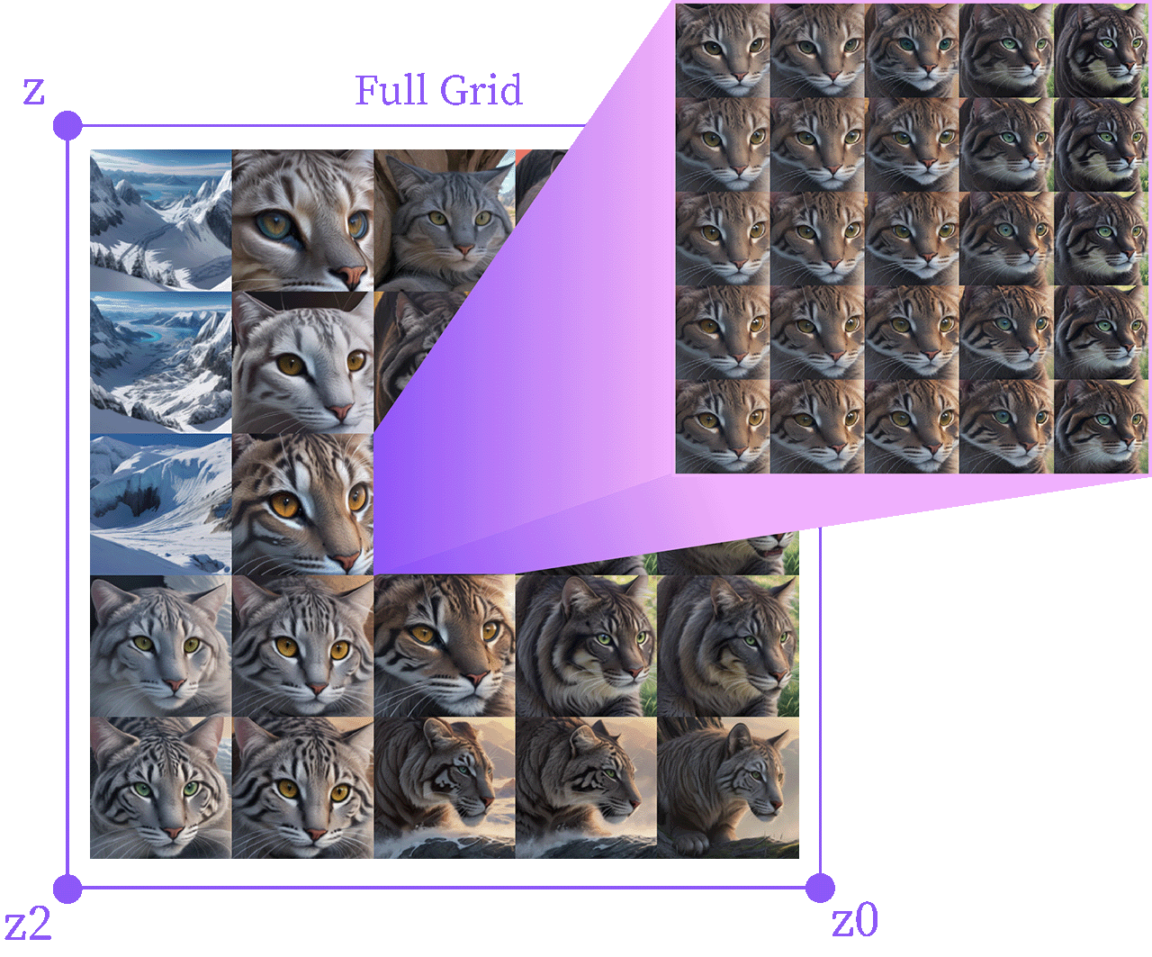
Following Lobashev et al. (2025), I spanned a grid in latent space to probe semantic boundaries, sampling up to 2,500 images across iterations. Three random latents \(z_0, z_1, z_2\) form the corners, from which a fourth point \(z\) is calculated via vector addition: \(z = (z_0 - z_1) + (z_0 - z_2)\). I then sampled the grid points by iterating through vector scalars \(α\) and \(β\) to obtain different position values for \(z\).
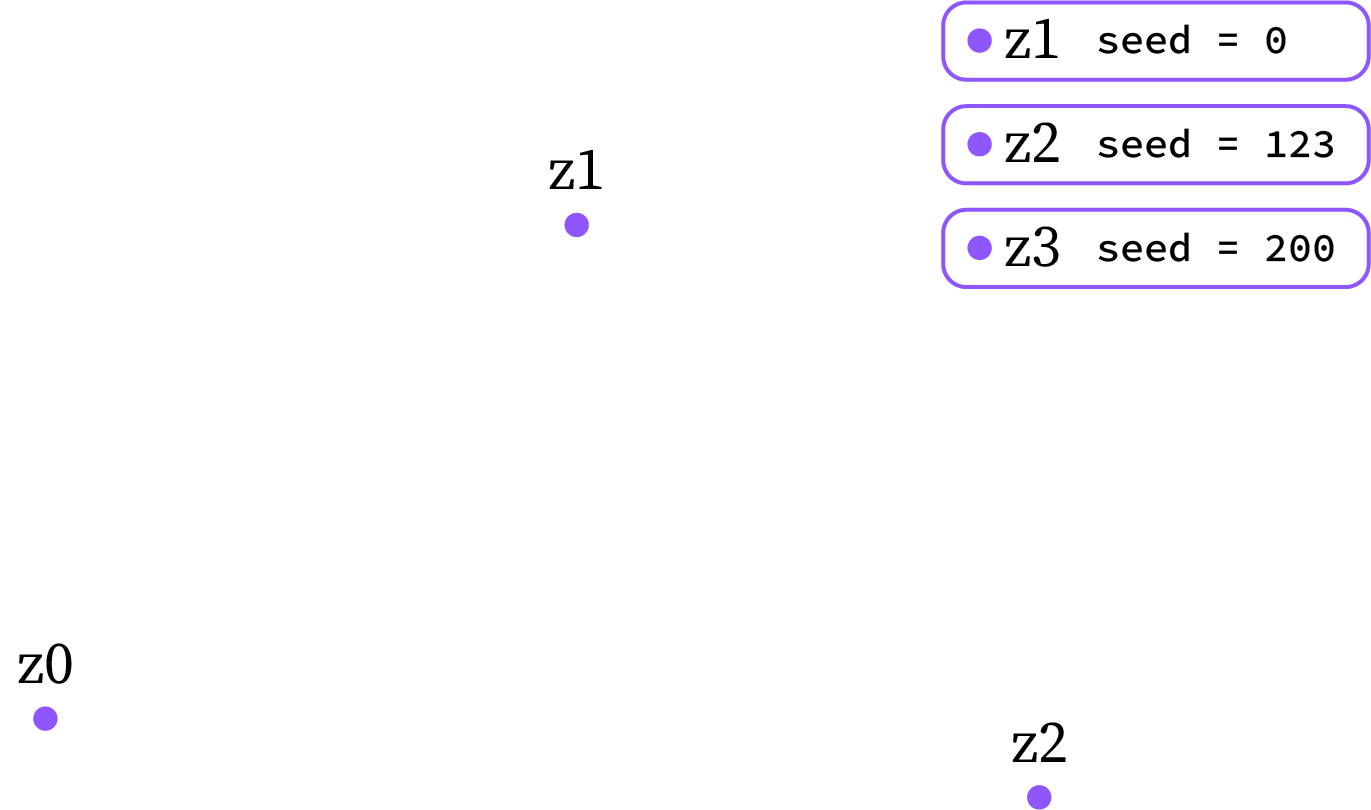
I started by generating three random latents. A latent is a compressed numerical representation of an image in latent space. It is 1/8 of the output image size, meaning a 64x64 latent results in a 512x512px image. We decode this latent through a diffusion pipeline.
Three random number generators are created with fixed seeds for repeatability. The latents created from these have the shape [1, 64, 64, 4], which represents a batch size of 1, the resolution, and 4 VAE channels encoding Gaussian noise that the diffusion pipeline decodes. The generated latent shapes are permuted into [1, 4, 64, 64], which a Stable Diffusion pipeline expects.
# Latent Paramters
latent_height, latent_width = 64, 64
latent_channels = 4

# Fixed Seeds
gen0 = torch.Generator(device=device).manual_seed(0)
gen1 = torch.Generator(device=device).manual_seed(123)
gen2 = torch.Generator(device=device).manual_seed(200)

# Random Latents
z0 = randn_tensor((1, latent_height, latent_width, latent_channels)
                  generator=gen0,
                  device=device,
                  dtype=torch.float16)

z1 = randn_tensor((1, latent_height, latent_width, latent_channels),
                  generator=gen1,
                  device=device,
                  dtype=torch.float16)

z2 = randn_tensor((1, latent_height, latent_width, latent_channels),
                  generator=gen2,
                  device=device,
                  dtype=torch.float16)

# Permuting Latent Shape for Stable Diffusion
z0 = z0.permute(0, 3, 1, 2)
z1 = z1.permute(0, 3, 1, 2)
z2 = z2.permute(0, 3, 1, 2)
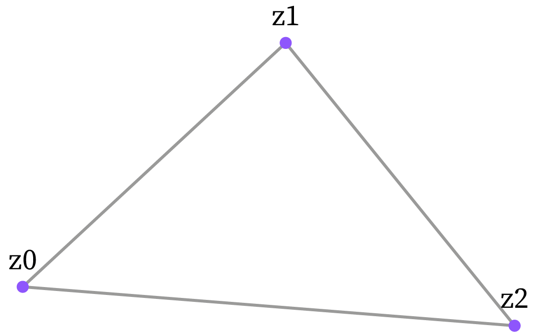
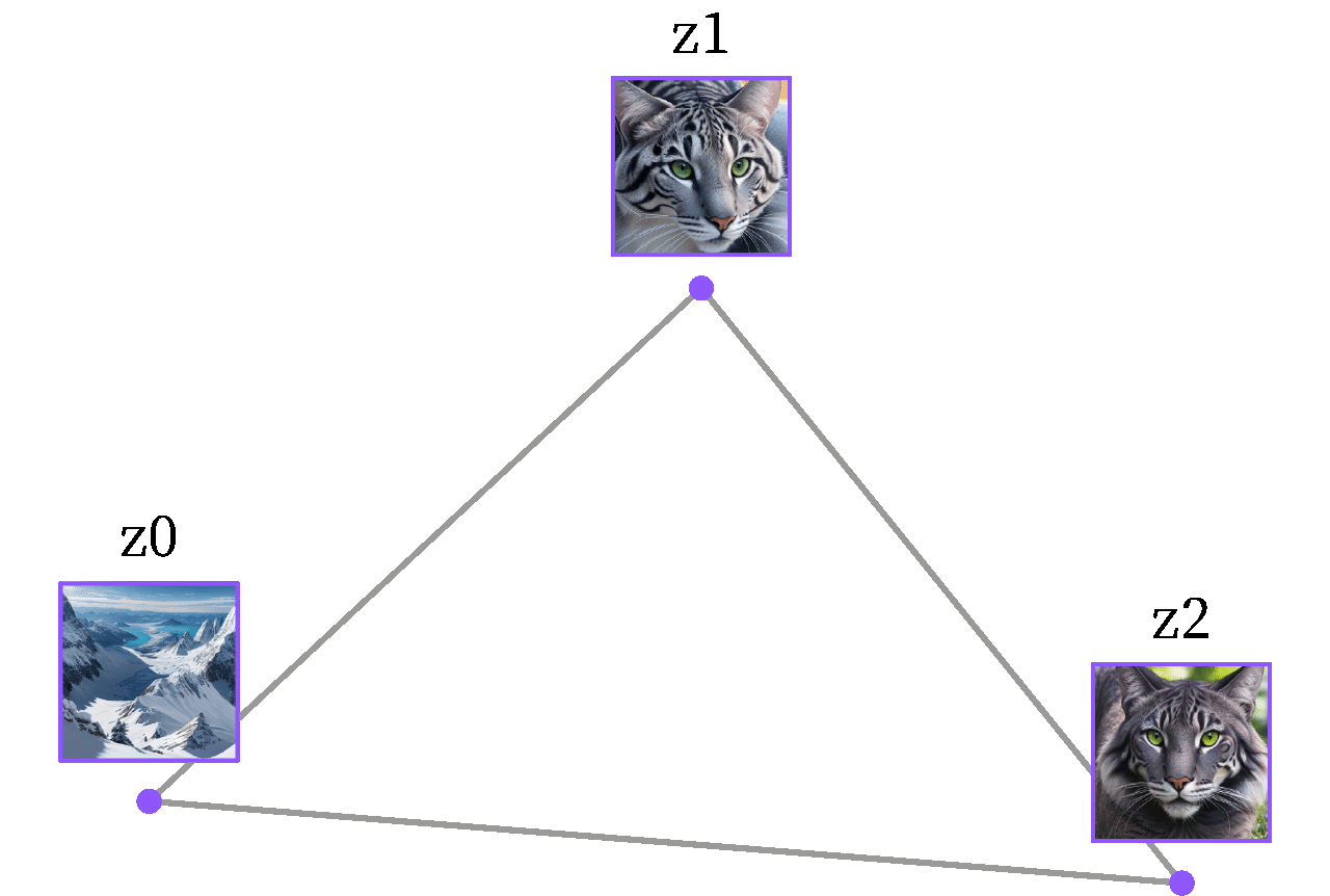
From the three base latents, a triangle naturally forms in latent space:
Decoding these corner latents via the replicated pipeline (\(η\)=0, CFG=5, 50 steps) immediately yields cats and mountains—strikingly similar to Lobashev et al. (2025), despite different random seeds.
Through linear combination \(z = (z_0 - z_1) + (z_0 - z_2)\) the triangle transforms into a parallelogram:
Introducing scalars \(\alpha\) and \(\beta\) for the vectors \((z_0 - z_1)\) and \((z_0 - z_2)\) respectively, enables to parameterize the space to find any point \(z\) through barycentric combinations of vertices \(\alpha, \beta \in [0,1])\).
\[z = z_0 + \alpha (z_1 - z_0) + \beta (z_2 - z_0)\]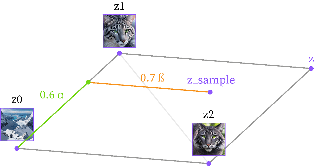
Decoding grid point \(z\) immediately reveals the first challenge: The reason the image looks this way is because raw latents require normalization to the VAE’s expected probability range to be decoded into a plausible image.
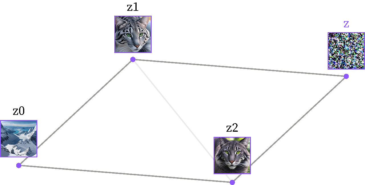
To fully understand what this normalization process does and to which point exactly the Latent gets normalized it is sensible to look into the math behind it.
Understanding Gaussian Hypersphere Normalization
Lobashev et al. (2025) note that diffusion models expect latents within a Gaussian probability space. Let’s build this intuition dimension by dimension.
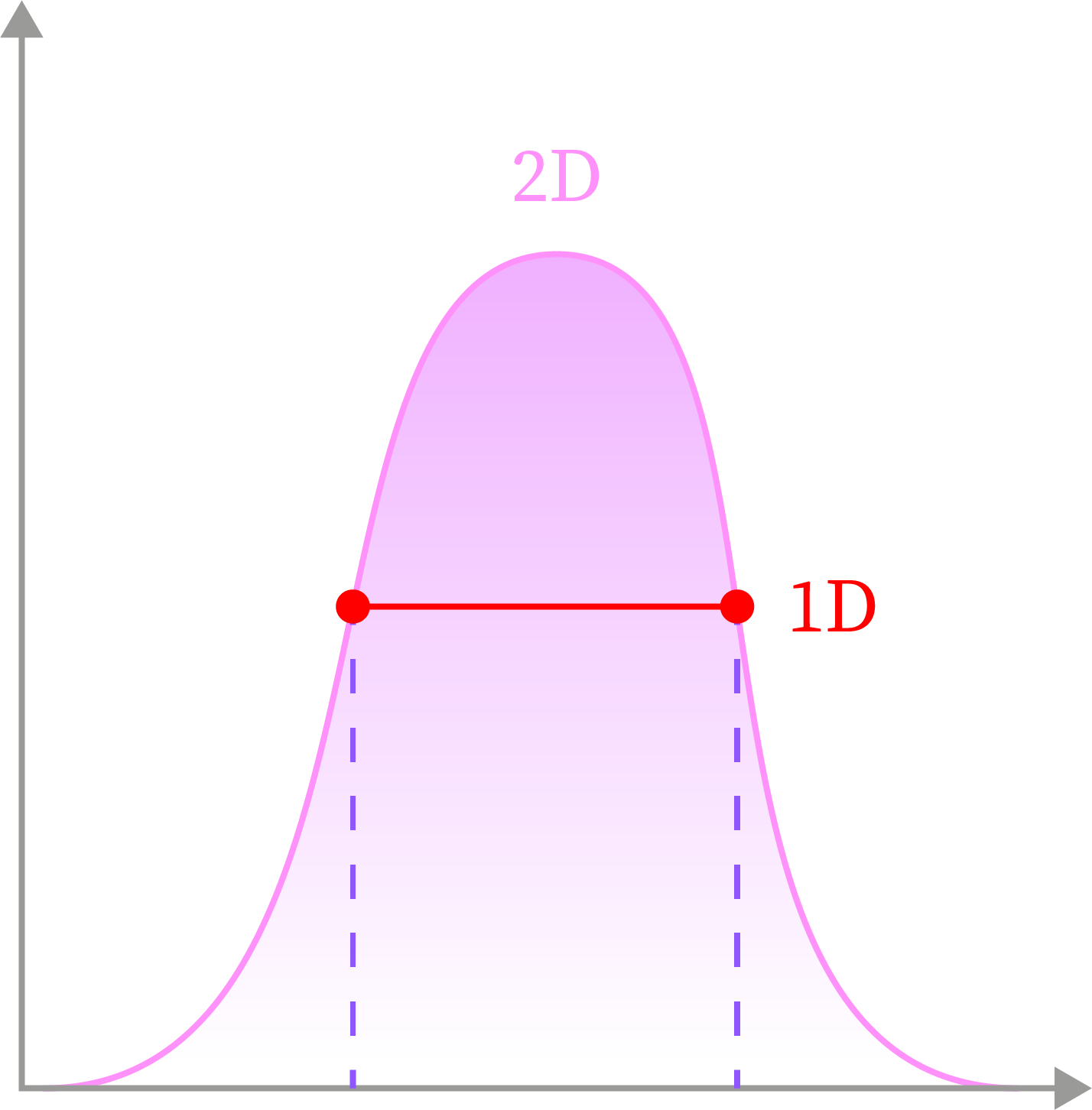
To understand what this means, let’s look at a 2D Gaussian distribution (the familiar bell curve). If we pick a specific probability value and ask, “Where else does this exact probability occur?”, we get a 1D contour line slicing through the peak. This is the set of all points sharing that probability density.
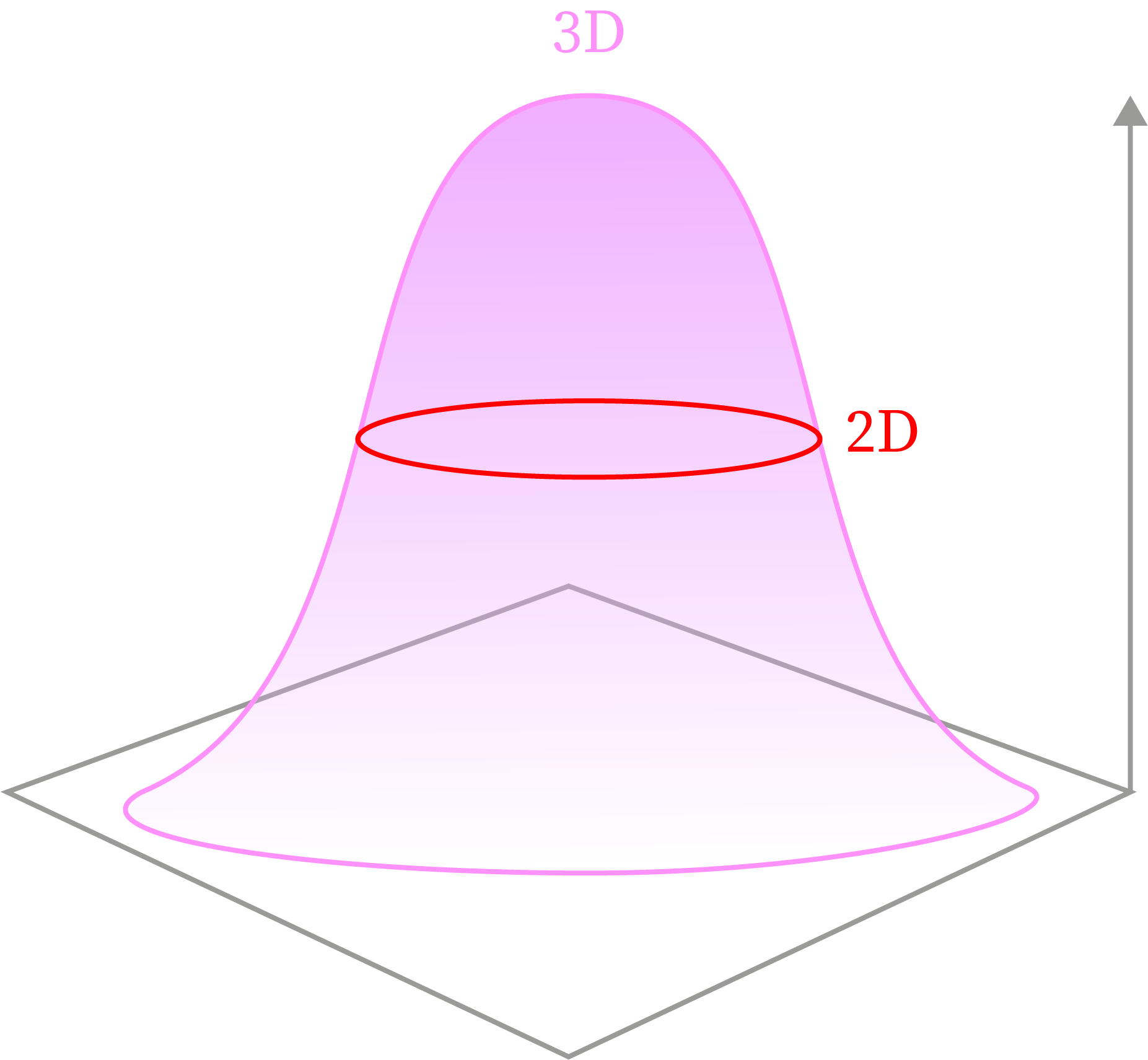
If we go up a dimension to a 3D Gaussian distribution. Now picking the same probability value, the answer forms a 2D circle.
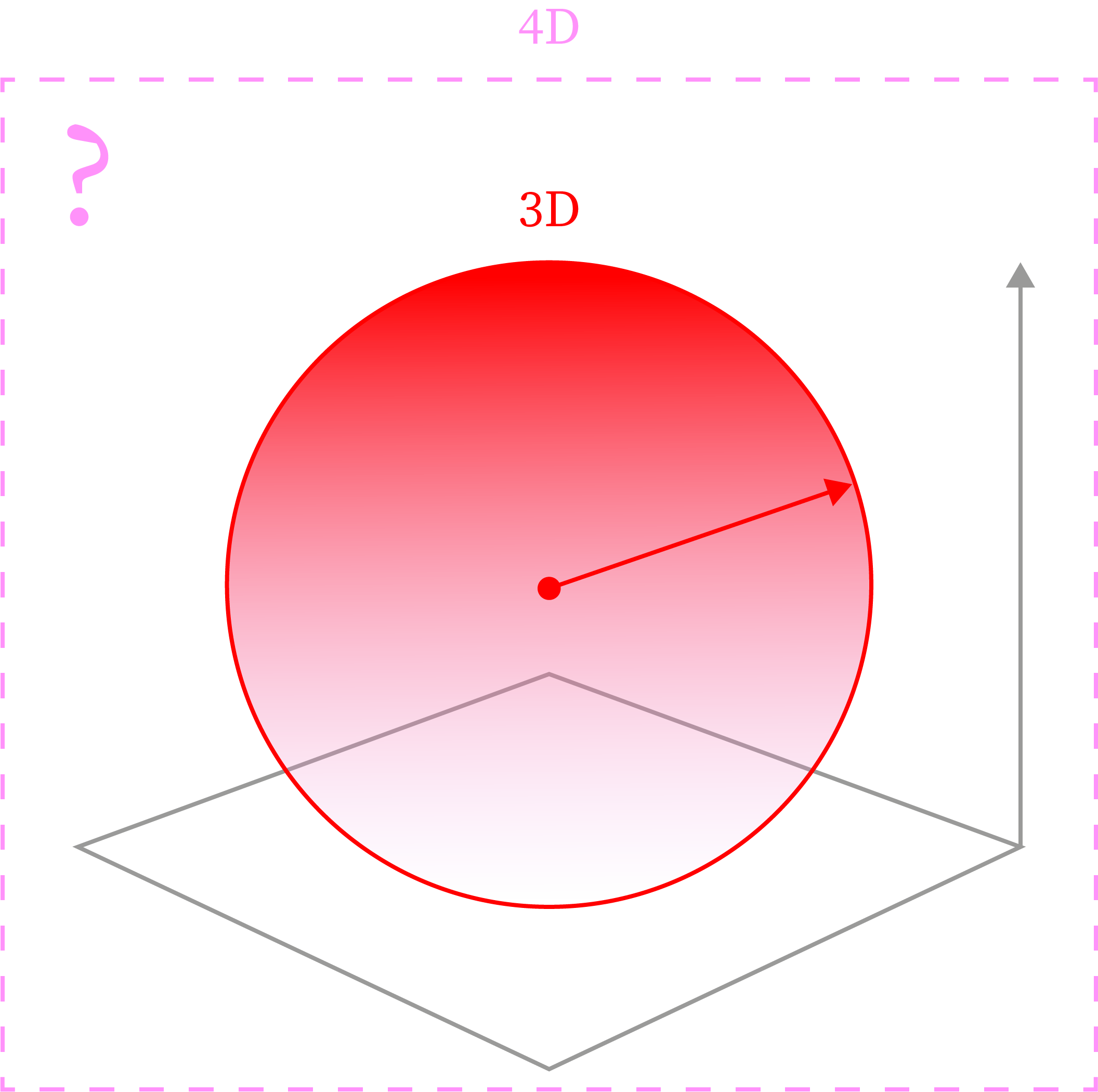
Increasing the dimension to 4D starts to lose the ability to depict the distribution. But the constant probability value now traces a 3D sphere.
Now what if we go even higher? Because Stable Diffusion doesn’t just operate in 4 dimensions. Accounting for the number of feature maps 4 and the latent resolution of 64x64, we get a dimensionality of \(4 \times 64 \times 64 = 16384\).
Extending the intuition from the previous examples, a constant probability value always exists one dimension lower than its Gaussian distribution. Thus, it resides in a space of \(16384-1\) dimensions.
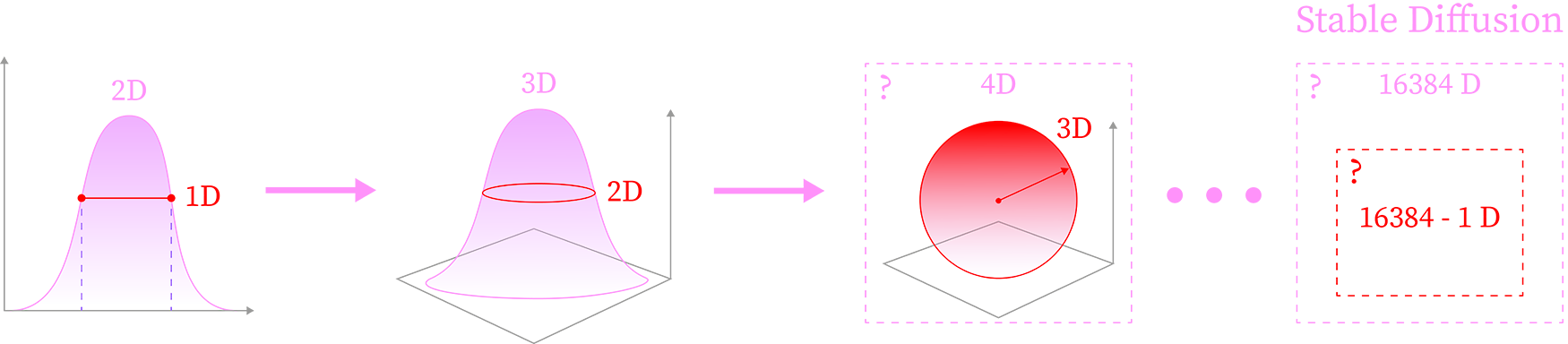
This constant probability value can again be depicted as a sphere for the simple reason that a vector equidistant from a center point at 0 in every direction can be visualized that way, even in spaces exceeding 16,000 dimensions. This structure is known as a Gaussian hypersphere or (d−1)-sphere (\(S^{d-1}\)).
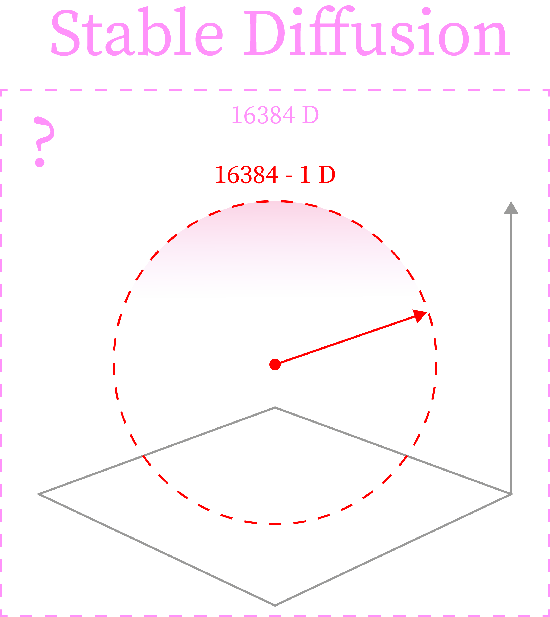
Thus latent vectors that are normalized to to this probability density value, can be decoded into plausible images. \(β\)
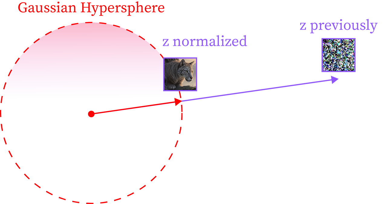
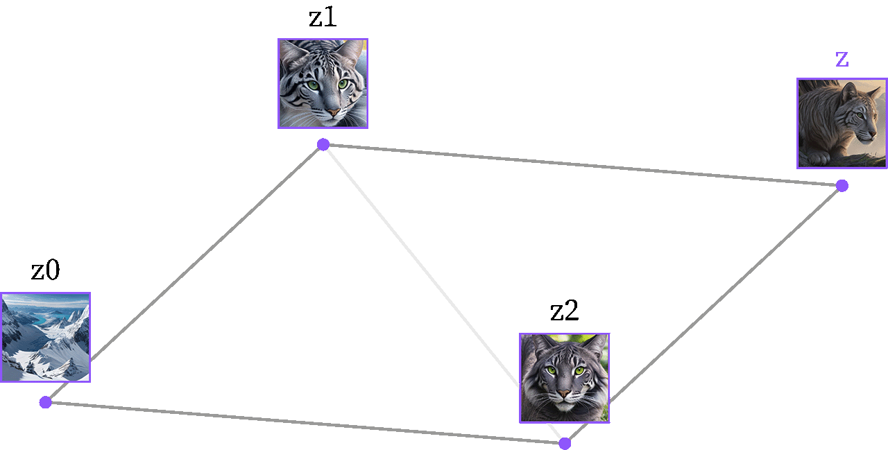
This raises a crucial question: If normalization to the Gaussian hypersphere was required for the calculated point \(z\) to produce plausible images, why did the latents \(z_0, z_1, z_2\) appear on it without any adjustment?
This is the latent that is constructed:
gen0 = torch.Generator(device=device).manual_seed(0)

z0 = randn_tensor((1, latent_height, latent_width, latent_channels)
                  generator=gen0,
                  device=device,
                  dtype=torch.float16)
A randn_tensor() usually has an even chance of being created at every point in a Gaussian \(\mathcal{N}(0,I)\). According to Gaussian Annulus Theorem, high-dimensional Gaussians like Stable Diffusion’s latent space defy 2D bell curve intuitions. While in low dimensions, probability mass clusters near the origin,
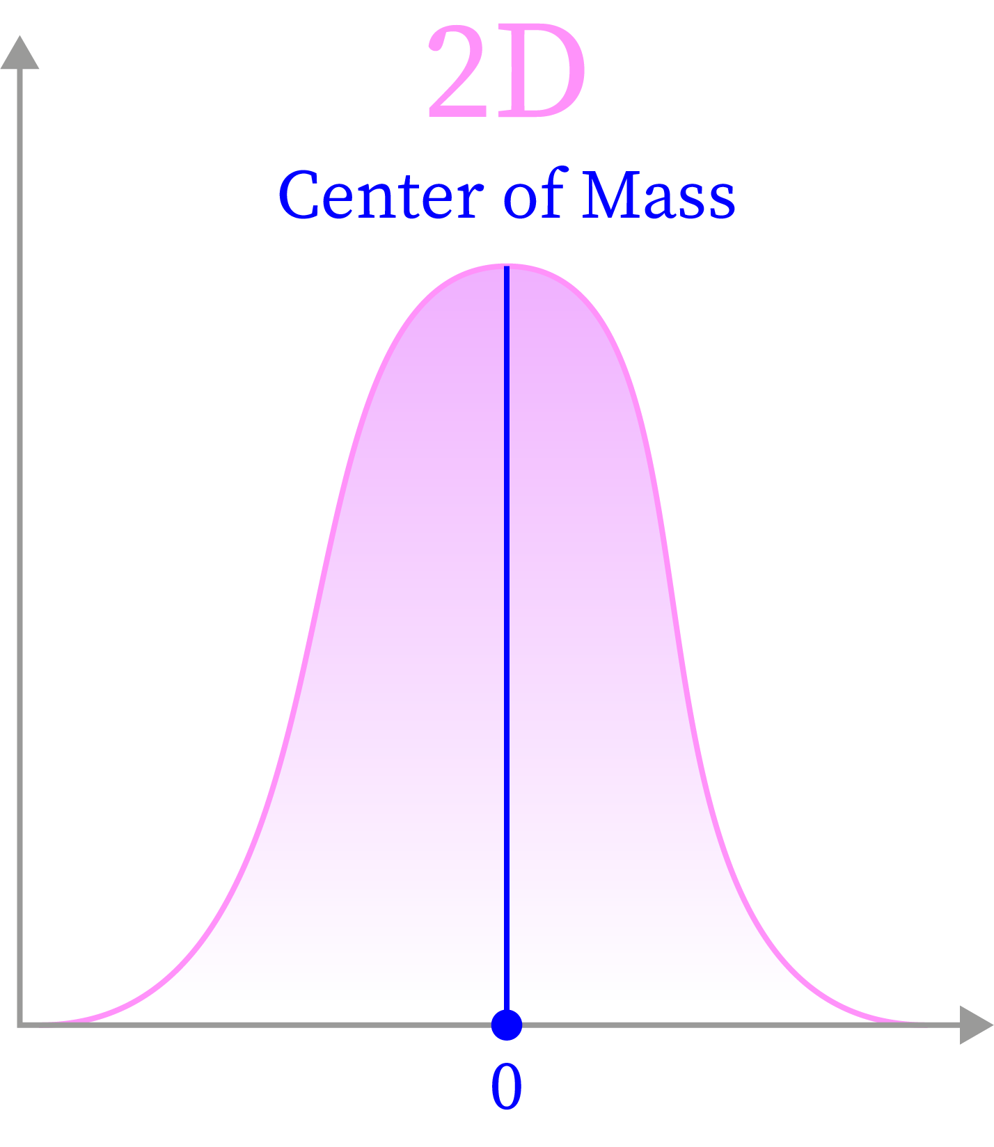
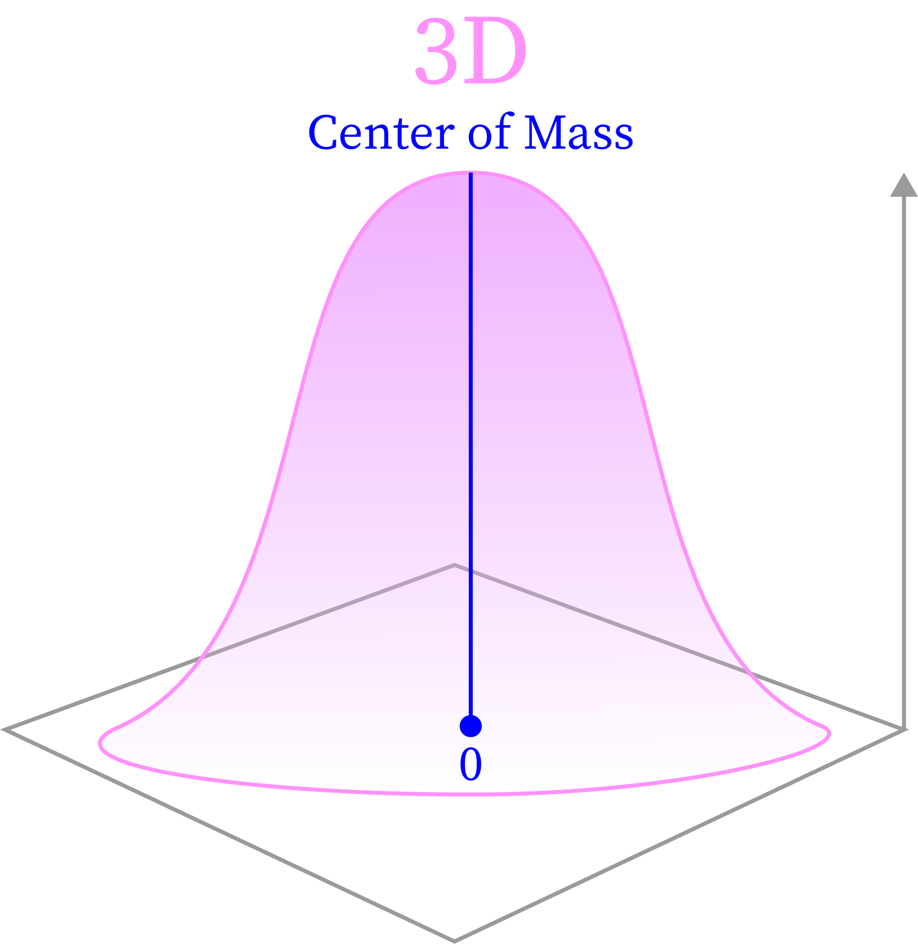
in high dimensions (\(d\gg1\)), nearly all probability mass concentrates in a thin shell (or annulus) around the center at a radius of approximately \(\sqrt{d}\) in \(d\)-dimensional space.
As dimension \(d\) increases, the annulus thins relative to the radius \(\sqrt{d}\). This “soap bubble” effect ensures that the vast majority of sampled points in \(\mathcal{N}(0,I)\) concentrate on the hyperspherical shell.
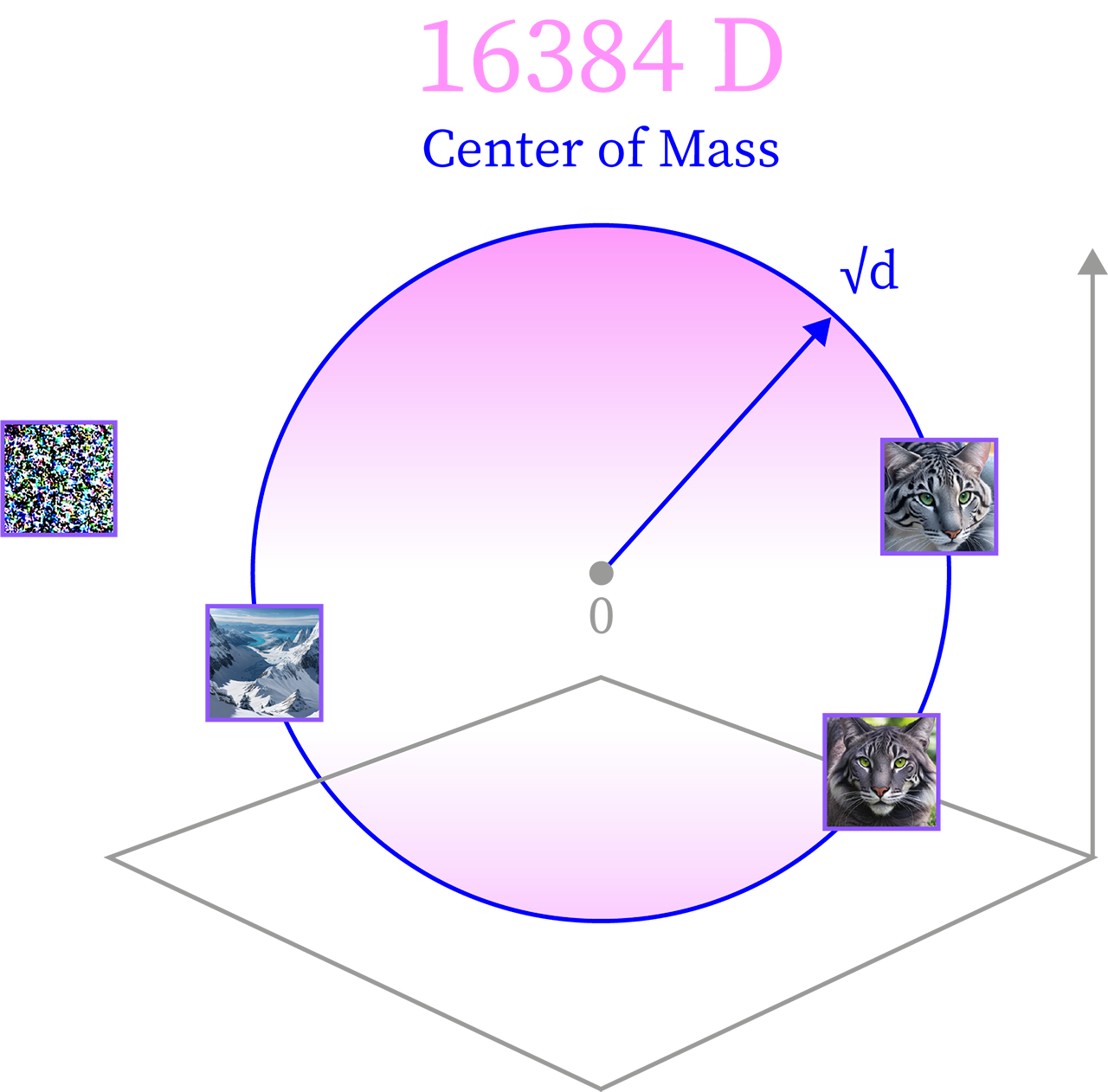
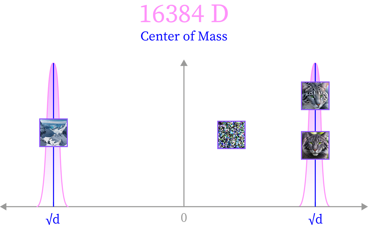
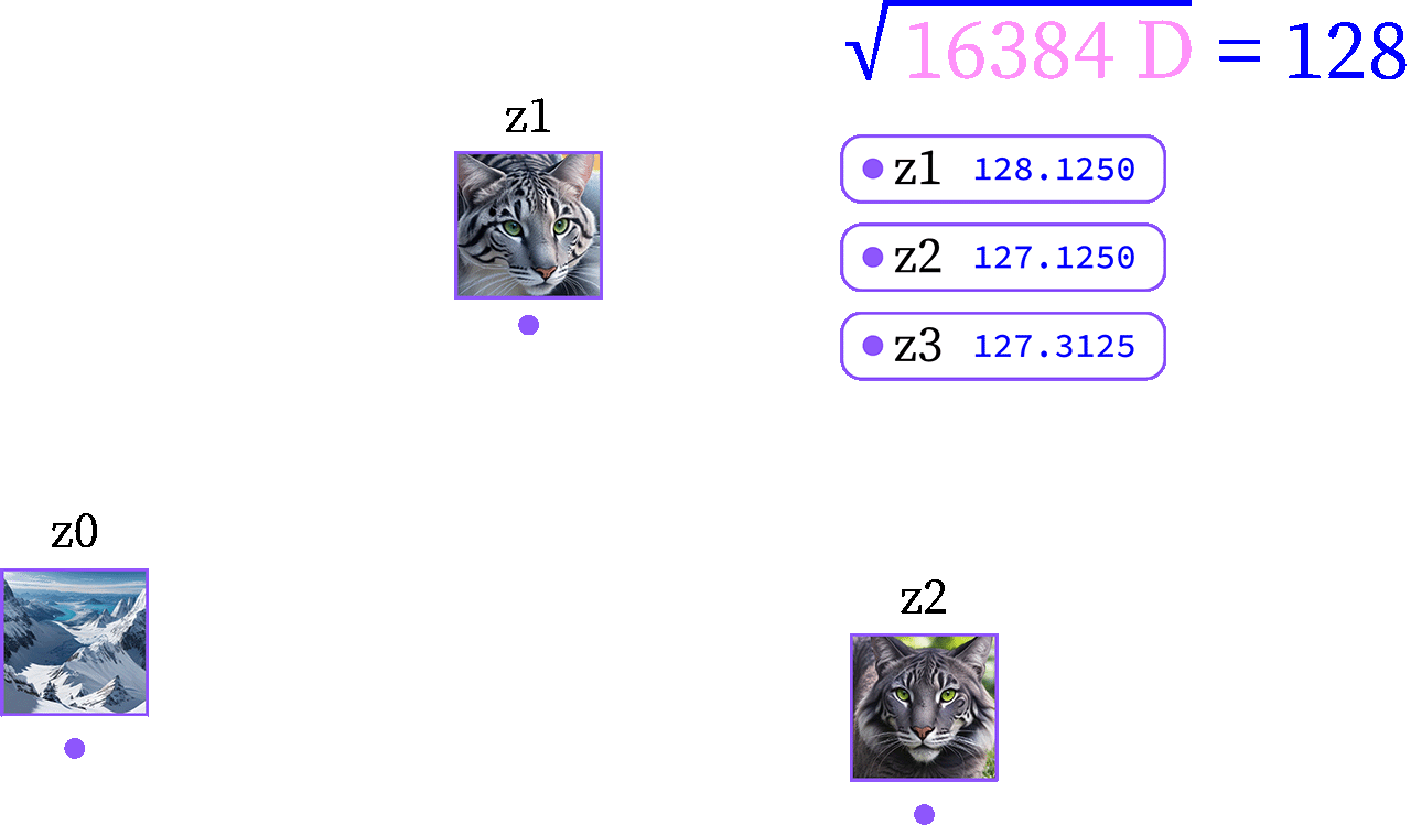
If applied to the latent space of Stable Diffusion, \(\sqrt{d} = \sqrt{16384} = 128\) using the tensor.norm() function, calculating the magnitudes of the latents \(z_0, z_1, z_2\) gives positions very close to the annulus.
| Latent | ∥z∥ | Distance from $\sqrt{d} = 128$ |
|---|---|---|
| \(z0\) | 128.1250 | +0.1250 |
| \(z1\) | 127.1250 | -0.8750 |
| \(z2\) | 127.3125 | -0.6875 |
While point \(z\), calculated through linear combination, drifts far outside: \(\Vert\mathbf{z}\Vert = 219.8750 \gg \sqrt{d}\). If normalized to \(\sqrt{d} = 128\), latent \(z\) will return a plausible image.
Sampling the Grid
By establishing a local target_norm from latents \(z0,z1,z2\),
# Local normalization target
local_target_norm = (z0.norm() + z1.norm() + z2.norm()) / 3
or calculating it from a separate latent, with torch.randn(1, 4, 64, 64) yielding a normalization target around 128,
# Global normalization target
example_noise = torch.randn(1, 4, 64, 64).to(device)
global_target_norm = torch.norm(example_noise).item() # ≈128
point \(z\) can be normalized and decoded into a plausible image.
With normalization solved, the parallelogram becomes fully decodable. Lobashev et al. (2025) sampled 60,000 points for exhaustive analysis; my home setup maxed out at 2,500, still revealing fractal rifts clearly.
Barycentric combinations generate any grid point \(z\):
\[z(\alpha,\beta) = z_0 + \alpha (z_1 - z_0) + \beta (z_2 - z_0)\]Nested loops iterate \(α, β ∈ [0,1]\) gridwise at the desired resolution (e.g., \(5\times5 = 25\) latents).
# Grid parameters
sampling_steps = 5
alphas = np.linspace(0, 1, sampling_steps) # alpha interval (rows/x)
betas = np.linspace(0, 1, sampling_steps) # beta interval (colums/y)

# Capturing latents and their metadata
latent_list = []
metadata_list = []

# Sampling latents
for idx_a, a in enumerate(alphas):
    for idx_b, b in enumerate(betas):

        # Sample latent
        z_sample = z0 + a * (z1 - z0) + b * (z2 - z0)

        # Normalize latent
        z_normalized = z_sample * (target_norm / z_sample.norm())

        # Create latent metadata
        latent_list.append(z_normalized)
        metadata_list.append({
            "filename": f"a{idx_a:03d}_b{idx_b:03d}.png",
            "row": idx_a,
            "col": idx_b,
            "alpha": float(a),
            "beta": float(b)
        })
Decoding each according to parameters set by Lobashev et al. (2025) to 512×512px images via the pipeline:
# Pipeline configuration
pos_prompt = "High quality picture, 4k, detailed"
neg_prompt = "blurry, ugly, stock photo"
inference_steps = 50
guidance = 5.0
pipe_seed = 42 # deterministic seed for reproducibility
pipe_generator = torch.manual_seed(pipe_seed)

for batch_idx, (latent_batch_linked, metadata_batch) in enumerate(batch_list):
    image_batch = pipe(
        prompt=pos_prompt,
        negative_prompt=neg_prompt,
        latents=latent_batch_linked,
        num_images_per_prompt=1,
        num_inference_steps=inference_steps,
        guidance_scale=guidance,
        generator=pipe_seed
    )
The result is for this example a 5x5 grid of images that can be sampled at a smaller area of interest for deeper analysis, by changing start and end points of the intervals for \(α\) and \(ß\).
Example adapted for sampling a 5x5 grid in the center for \(α, β ∈ [0.4,0.6]\):
sampling_steps = 5
alphas = np.linspace(0.4, 0.6, sampling_steps) # alpha interval (rows/x)
betas = np.linspace(0.4, 0.6, sampling_steps) # beta interval (colums/y)
Batching Pipeline Optimization
To accelerate grid exploration, I implemented GPU batching, processing multiple latents in parallel through single U-Net forward passes per denoising step. On 24GB VRAM (RTX 4090), a batch size of 8-12 hits the sweet spot, reducing per-image reverse diffusion from 2s to 0.3s (6.7× speedup).
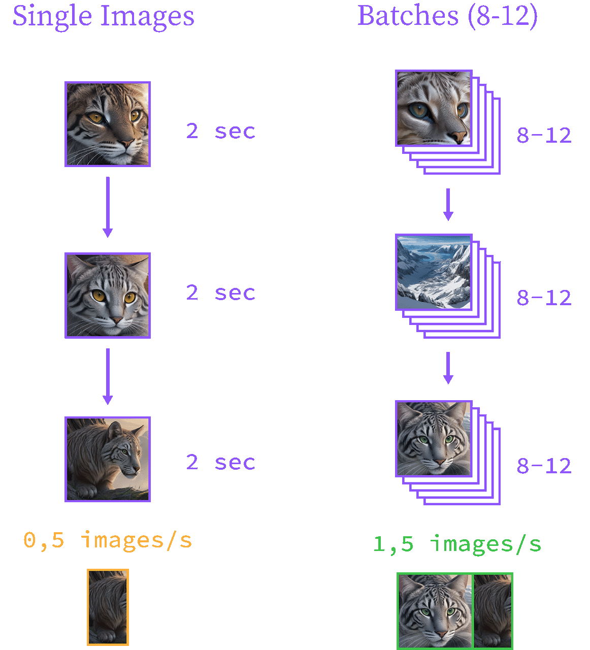
Latents reshape from single [1, 4, 64, 64] to batches (e.g., for batch size 8) [8, 4, 64, 64] via concatenation along the batch dimension, with metadata (\(α, β\) coordinates) tracked for reconstruction. Processed batches are stored as (latent_tensor, metadata) tuples and passed to the pipeline.
batch_list = [
    (tensor_batch_1, metadata_batch_1),  # [8, 4, 64, 64], ["α=0.0 β=0.0", ...]
    (tensor_batch_2, metadata_batch_2),  # Batch 2
    ...
]
To avoid token mismatch between the latents and the text prompts for U-Net cross-attention, the number of text-embedding tokens must match the tokens in the batch. While single latents have \(4,096\) tokens (\(1\times64\times64\)) matching text embeddings, batches (e.g., 8) scale to \(32,768\) tokens (\(8\times64\times64\)). For a dynamic pipeline ensuring token parity for parallel denoising, I set num_images_per_prompt to match the batch_size of the latent tensor.
# Pipeline parameters (paper configuration)
pos_prompt = "High quality picture, 4k, detailed"
neg_prompt = "blurry, ugly, stock photo"
inference_steps = 50
guidance = 5.0
pipe_seed = 42 # deterministic seed for reproducibility
pipe_generator = torch.manual_seed(pipe_seed)

# Pipeline
for batch_idx, (latent_batch_linked, metadata_batch) in enumerate(batch_list):
    image_batch = pipe(
        prompt=pos_prompt,
        negative_prompt=neg_prompt,
        latents=latent_batch_linked,
        num_images_per_prompt=latent_batch_linked.shape[0], # accounts for batchsize
        num_inference_steps=inference_steps,
        guidance_scale=guidance,
        generator=pipe_seed
    )
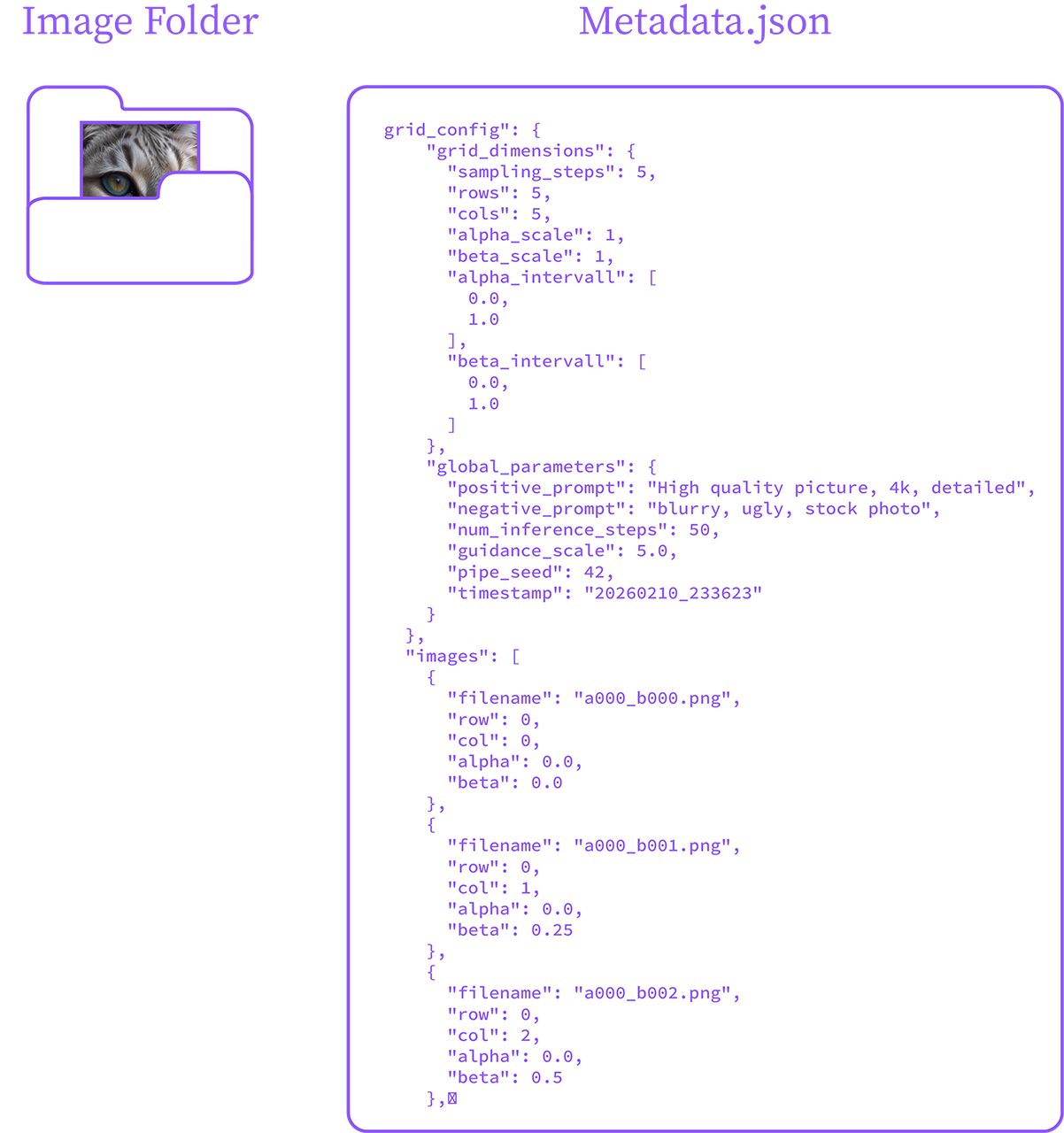
The resulting images are exported to disk, with an accompanying metadata.json file that records global configuration, including grid resolution, prompts used, and the positional coordinates of each latent within the grid.
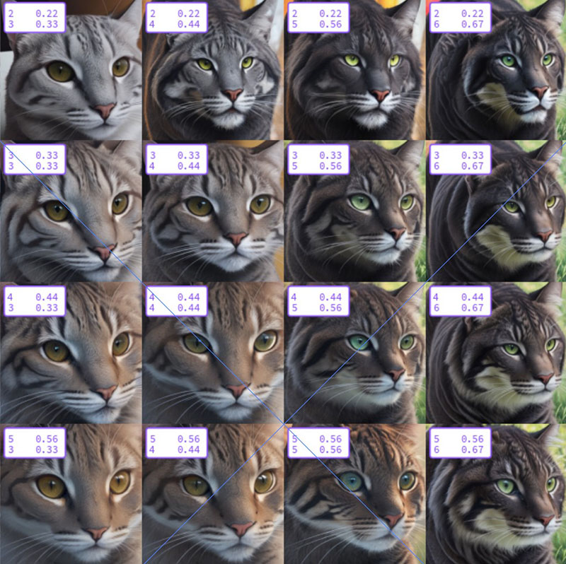
Leveraging the metadata.json positional data, Matplotlib visualizes the latent grid with dual annotations: grid indices (\(x, y\) intervals) and parameter coordinates (\(\alpha\), \(\beta\)) for each point.
Results: Mapping Semantic Fractures
Initial Rift discovery
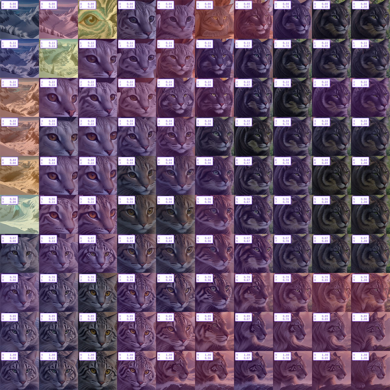
Increasing the grid resolution to 10×10 (100 images) exposes the first anomaly: a hybrid form blending both mountain and cat features, failing to resolve into either concept. This could be indicative of the phase transitions discussed in the paper.
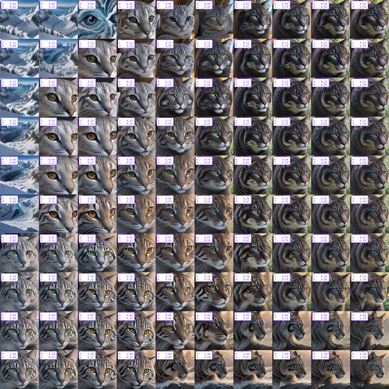
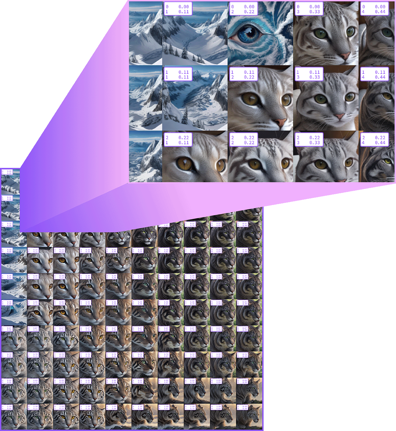
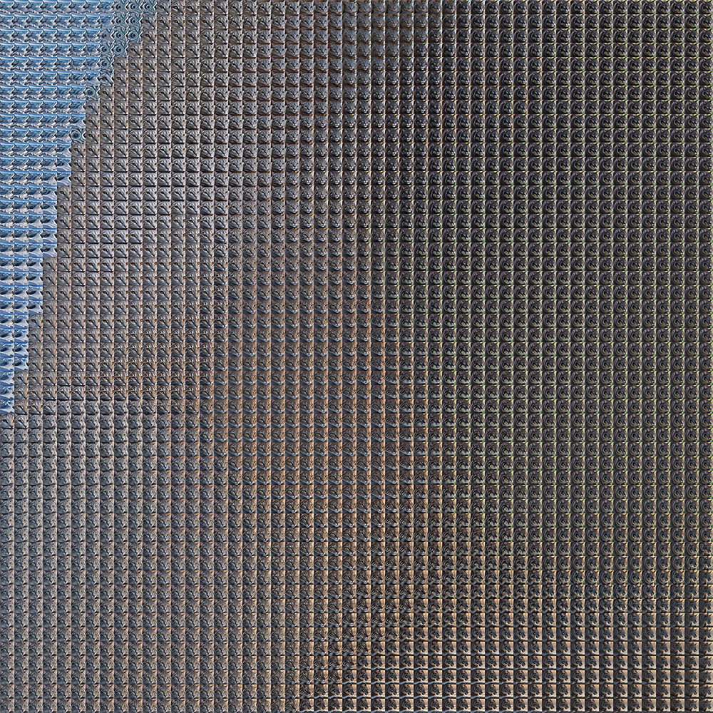
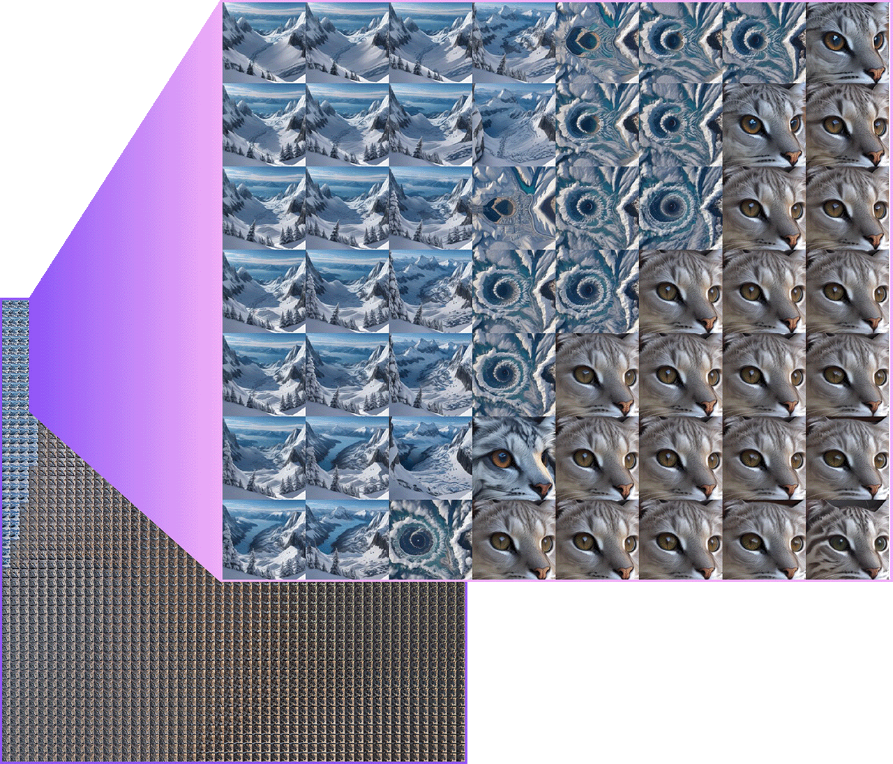
At 50×50 resolution (2,500 images), the semantic rift crystallizes: a sharp boundary separates stable cat ↔ mountain domains, with fractal instability concentrated at the transition’s northern edge, where the anomaly was spotted.
CLIP Lipschitz Analysis
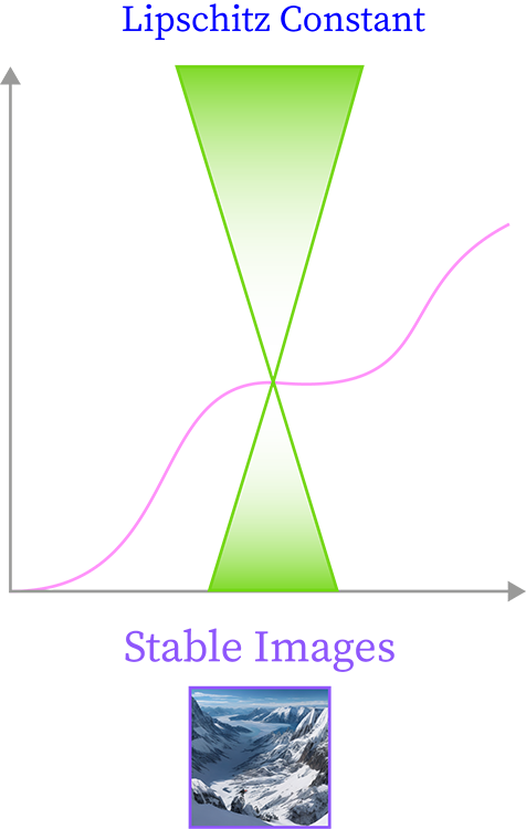
Lobashev et al. (2025) rigorously quantify this geometry. To detect the distinct phases, they trained a neural network on the log-partition function to reconstruct the Fisher information metric of the space, which had discontinuities along the borders between concepts. Through this approach, they calculated geodesic paths between semantic domains, achieving smooth interpolations. To quantify model instability at transitions, they used the Lipschitz constant—a measure tracking the rate of change of a function. At phase boundaries, this constant diverges, suggesting extreme fluctuations in model output resulting from only small changes to the input latent vector, even at scales of \(10^{-8}\) (the model’s resolution at half-precision bit level).
Each grid image is fed through CLIP’s image encoder to extract image features yielding high-dimensional semantic fingerprints describing the content of the image.
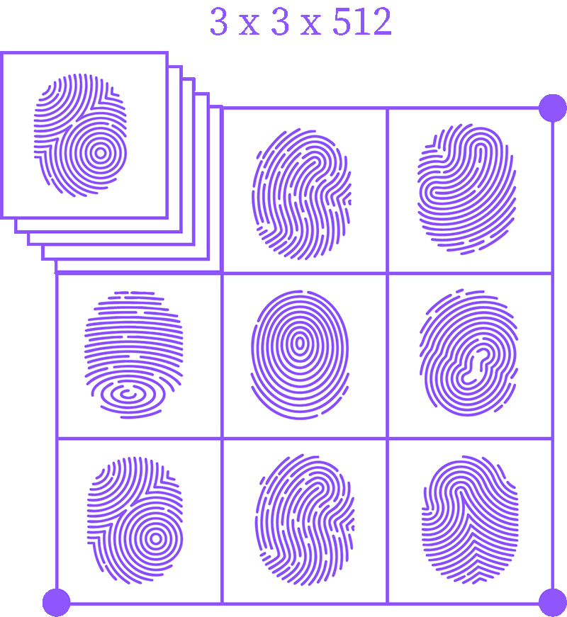
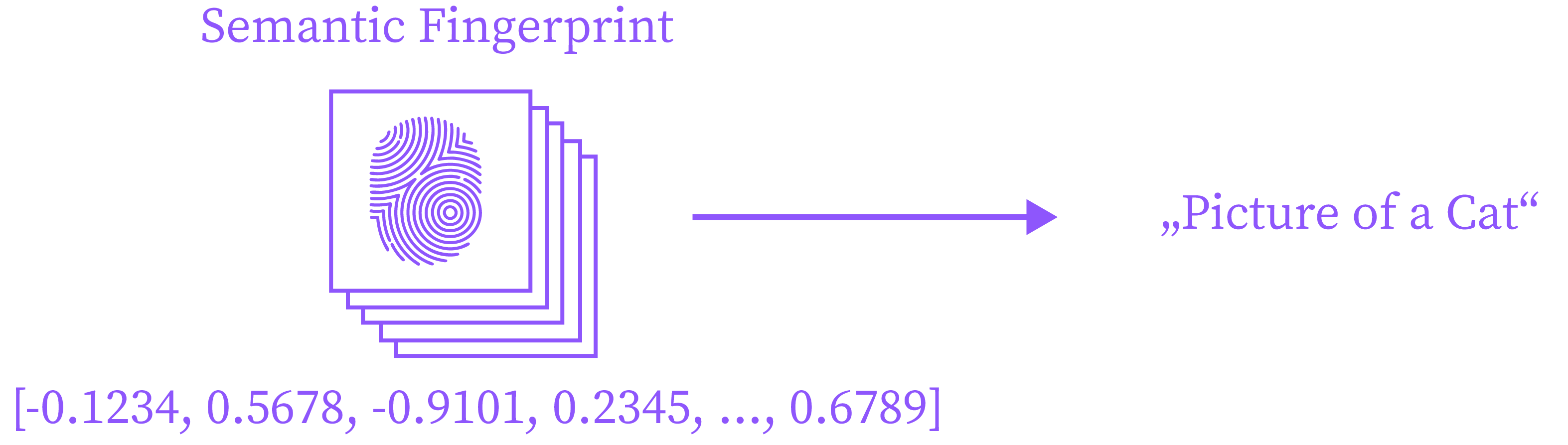
These fingerprints are formed into a feature map that preserves the original (\(\alpha, \beta\)) coordinates. This feature map is analyzed for local gradient magnitudes across horizontal and vertical axes, then used to compute the Lipschitz constant, which measures output sensitivity between grid neighbors.
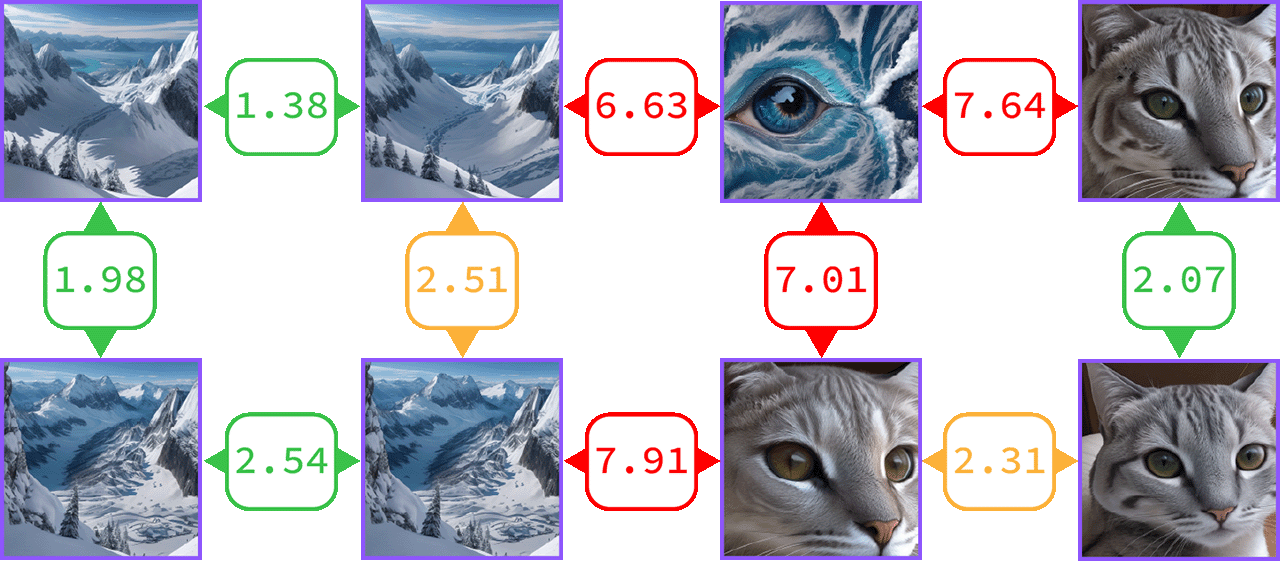
Each cell’s Lipschitz amplitude is averaged across neighbors, yielding a stability field overlaid on the original grid. Rift regions show explosively high values, confirming extreme sensitivity where concepts collide.
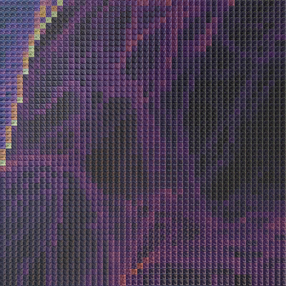
The Lipschitz field reveals phase divergence in clear detail. A sharp border cleanly separates mountain and cat manifolds, peaking at the fractal rift where model coherence collapses.
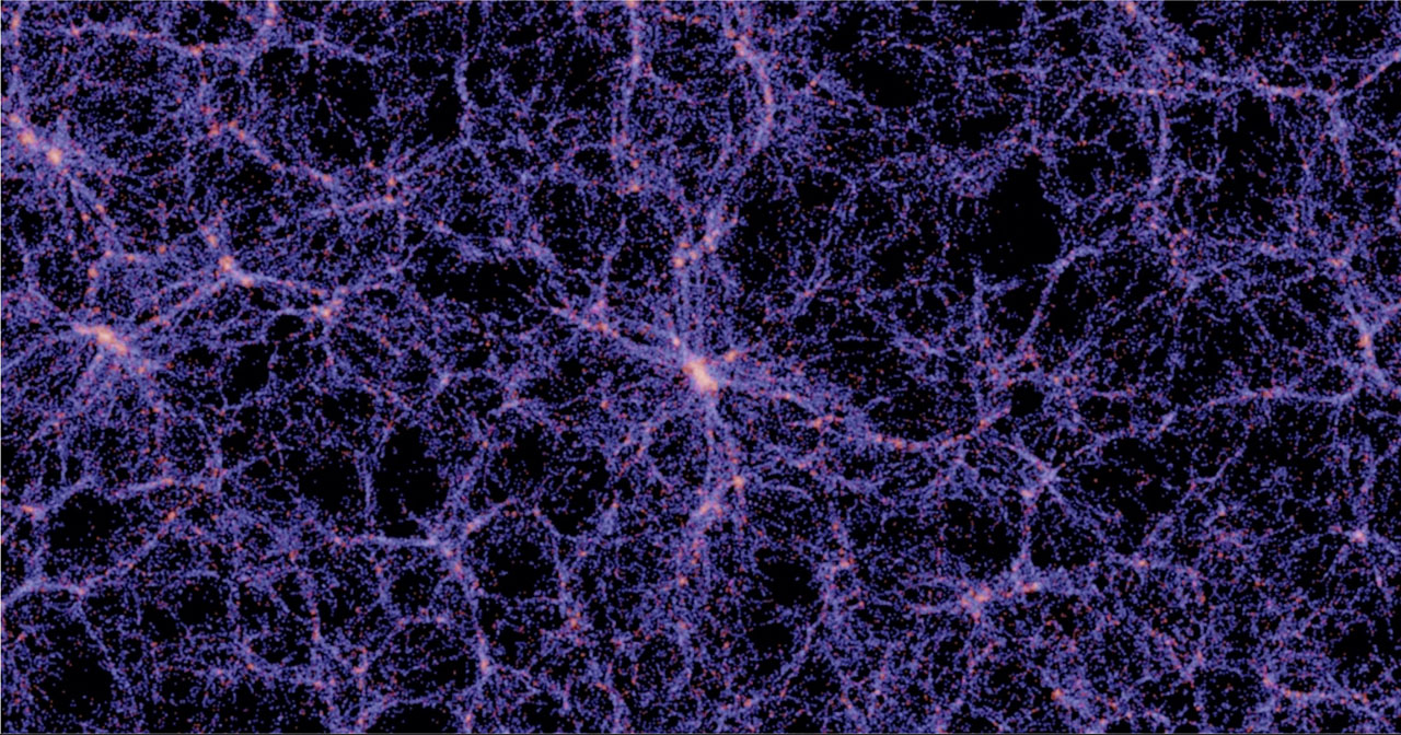
The resulting structures are quite stunning. They distinctly remind me of mappings of cosmic voids—vast galaxy-free bubbles ringed by dense clusters, born from gravitational instabilities that cause matter to clump. Speculatively, latent space could similarly enforce its “semantic gravity,” which pulls images toward stable concepts, leaving rifts at the unstable frontier.
The bit-level Lipschitz divergence is reproducible and confirms Lobashev et al. (2025)’s observations. Now we shift to the project’s purpose: exploring what novel forms might emerge from these semantic voids.
Exploration: Finding novel Image output
Encoding Images to Grid Vertecies
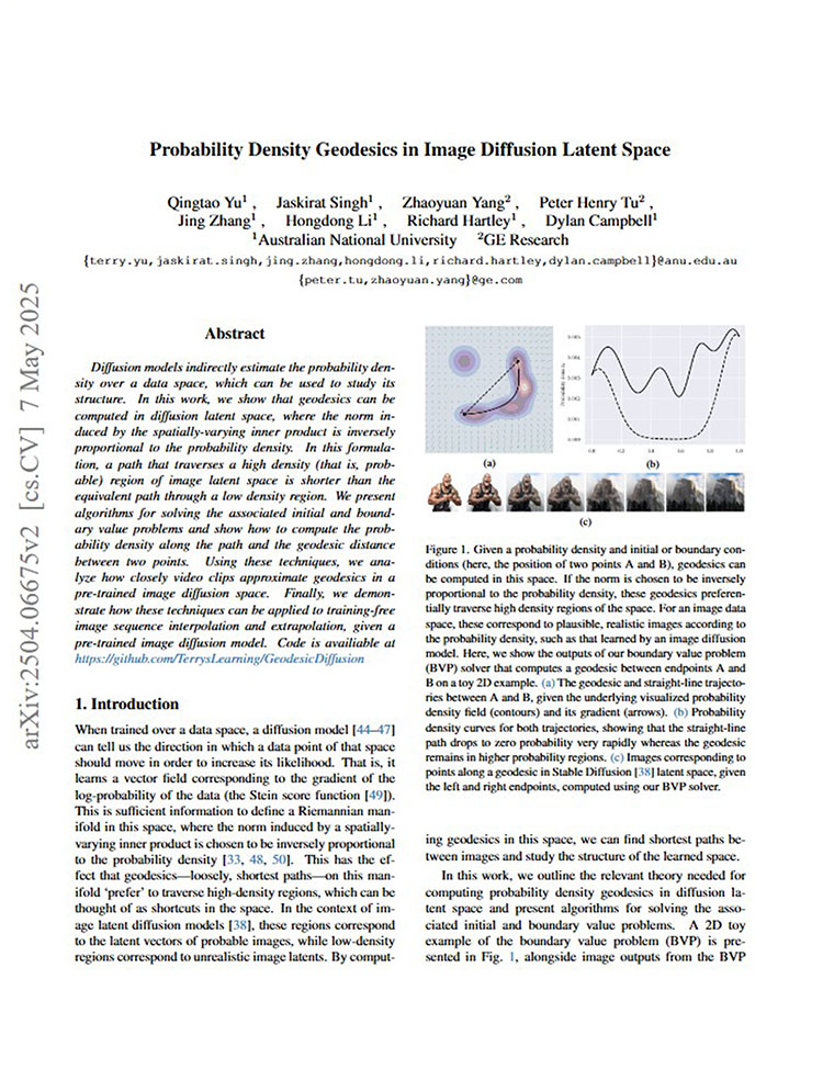
Inspired by these fractal rifts, I explored image-derived grid vertices. Yu et al. (2025), in Probability Density Geodesics in Image Diffusion Latent Space, tackle similar latent geometry challenges, developing methods to encode existing images and trace interpolations between them. I was particularly amused by their example of interpolating between actor Dwayne “The Rock” Johnson and a literal rock.

This echoed a conversation with a middle school art teacher friend, who introduced her class’s “Symbiosis” project: students chose two contrasting texture patches and glued them onto a sheet of paper, then hand-drew the space in between. A form of manual interpolation.
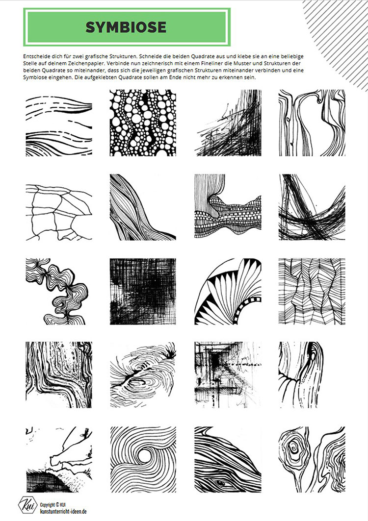
What sparked my interest was the idea of encoding these texture patches as latent vertices and then comparing the resulting interpolation grid with their human-drawn counterparts.
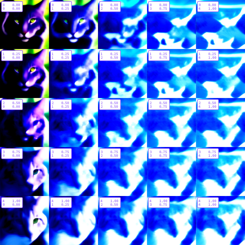
Initial experiments hit a hard limit. It seemed that either my encoding or decoding approach was flawed, resulting in malformed image diffusion. Even importing the original “cat/mountain” images from previous experiments proved troubling. This wall seemed intractable for now, so I decided to revisit it later with the necessary knowledge and focus first on a different approach.
Exploring Concepts beyond neutral prompts
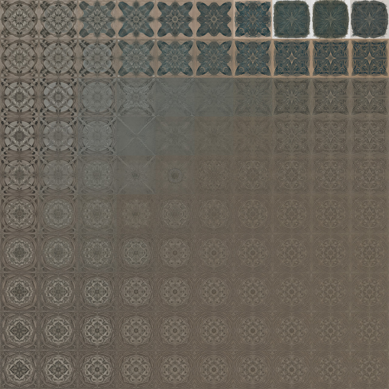
Abandoning image-derived latents, I pivoted to prompt-guided rift diving within the validated random latent parallelogram formed by \(z_0, z_1, z_2, z\), replacing Lobashev et al.’s (2025) neutral prompts (“high quality picture”) with more concrete ones to reveal interesting image spaces.
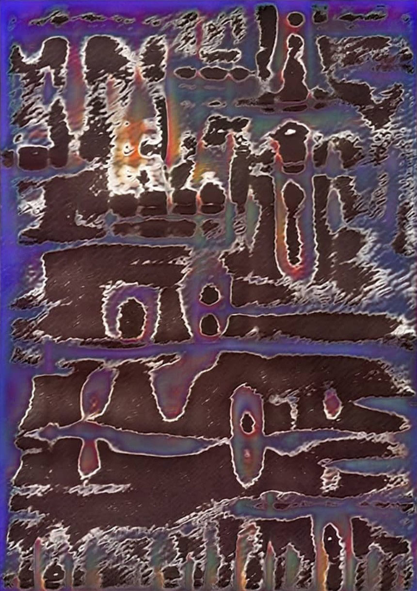
Here is an exploration of textures and ornaments:
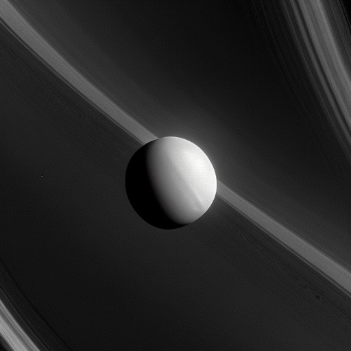
What sparked my interest the most was the metaphor of discovering the latent space being similar to discovering the universe like a satellite.
A notable video is the uncut stream of all 341,805 images of the Cassini’s Saturn mission (2004-2015) endures with mesmerizing, eerie quality, depicting space as almost Lovecraftian.
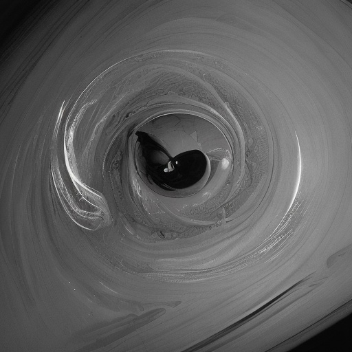
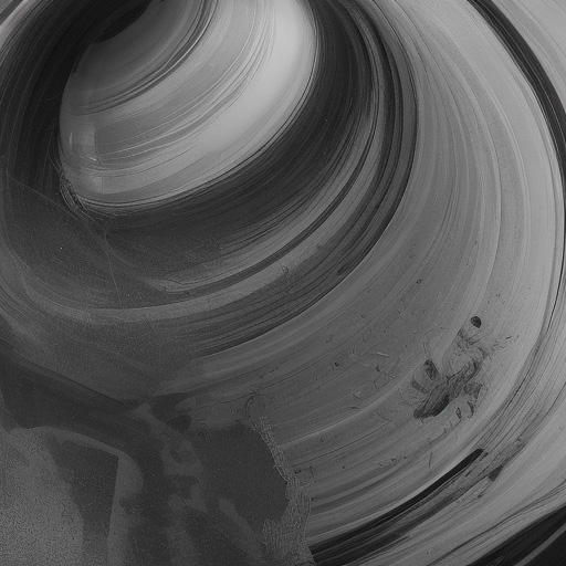
positive prompts: “NASA Cassini spacecraft image of Saturn in greyscale with intricate rings casting sharp shadows, distant moons like Enceladus and Titan visible, > realistic colors, scientific photography, high resolution, from orbit, dramatic lighting from sunlight, vast space background, artifacts”
negative prompts: “centered subject, stock photo, person, ornament, fantasy, colorful, flashy”
With the depicted prompts, I sampled the grid for novel discoveries. Trying to push the fringes of the model, I started pushing scalars \(\alpha, \beta\) to (10×–1000×) their range, catastrophically breaking Gaussian hypersphere projection. Latents drifted to \(\lvert \mathbf{z} \rvert \gg 128\), yielding undecodable noise. A space where, to stay with the metaphor, latents escaped the observable universe into the incoherent void.
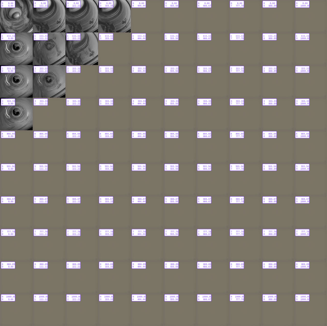
Some of the resulting fringe images revealed an uncanny beauty, in my opinion.
Reflection
This research project taught me to overcome my hesitation in reading AI and ML papers for true understanding and in looking up and implementing mathematical theorems. Replicating a paper’s process forced me to pay attention to the details and ensure everything ran correctly. While it strengthened my perspective on the mathematical and data-driven aspects of a project, I find the most fulfillment when I can combine these elements with concepts I am personally passionate about. I hope to incorporate some of these lessons into my master’s thesis, which I plan to pursue after my break semester, when I will have a clearer preview of the topic I want to explore.
References
Lobashev, A., Guskov, D., Larchenko, M., & Tamm, M. (2025). Hessian Geometry of Latent Space in Generative Models. arXiv link
Yu, Q., Singh, J., Yang, Z., Tu, P. H., Zhang, J., Li, H., Hartley, R., & Campbell, D. (2025). Probability Density Geodesics in Image Diffusion Latent Space. arXiv link
“11 Years of Cassini Saturn Photos in 3h 48min” (n.d.). YouTube video
Recommended citation: Mehl Ricardo, You. (2026). "LatentWorld: Exploration of Latent Space Phase Transitions as a way of generating novel Images Number 1." Journal 1. 1(1).
Download Paper | Download Slides | Download Bibtex